Click here for the Learning Curve in PDF format.
The Local Correlation Model
Many ideas have been proposed to build correlation smile curves close to those observed in the tranched iTraxx market. More recent research has focused on making correlation a random variable itself, for example by making it a function of the economy. In mathematical terms, such models are known as Gaussian mixtures. A popular assumption has been to change the beta of each single issuer according to whether the state-of-the-economy factor is above a given threshold. This last approach seems the most promising to us, but it relies on a wide range of hidden parameters, making the model quite unstable when it comes to pricing derivative products such as CDO squared. We propose alternatively to adopt a descriptive approach and to start from market observations to specify the correlation model.
The key idea of our model is to make correlation a function of the economy. In this view, it is similar to the up and down model mentioned above. There is a striking difference, however: correlation is supposed to be a smooth and homogeneous function of the economy. A deterioration in economic fundamentals affects all issuers at the same time and gradually.
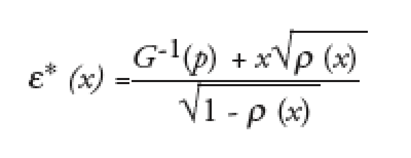
In mathematical terms, we decided to use the same correlation * for all names, and to make correlation a function *(X) of the economy:

In the standard Gaussian copula framework, * is constant and does not depend on X. In our framework however, one can use the same numerical approach as in the Gaussian copula framework once the * dependence on X has been computed.
The distribution of portfolio losses needs to be adjusted to take into account the whole base correlation smile
As we have mentioned above, the base correlation and the compound correlation approaches are not coherent frameworks. The market prices CDOs based on a perception of risks that is not the one involved in the traditional Gaussian copula model. Intuitively, a steep skew points to a sharp increase in risks on higher strikes.
For European CDOs, (i.e. CDOs that pay the premium whatever the outcome on credit events) there is a smart formula for estimating directly the market-implied distribution of losses given the base correlation skew. This formula gives an adjustment to the naïve distribution of losses that can be computed using only one point of the base correlation skew:

where L(K) is the distribution of losses in the portfolio, L(K,* ) is the naïve distribution using the base correlation * for the given strike K that we note, Skew(K,* ) is the skew of the base correlation curve at strike K and Rho(K,* ) is the sensitivity of the portfolio loss to a change in base correlation.
We call this relationship the market law of losses. It makes the link between the distribution of losses within the Gaussian setting used for pricing CDOs, and the distribution of losses really implied by the whole correlation structure.
The individual asset value law is no longer Gaussian
If we take an homogeneous portfolio, all the names have an identical default probability function p(t). All their asset values Aj have the same cumulative function G. This function is the Gaussian cumulative function in the Gaussian copula framework. It is not the case anymore in the local correlation framework and it is equal to:

This formula shows that G depends on *. Therefore one needs a process to find G and the local correlation function *(X) jointly.
From Portfolio Loss To Local Correlation
We have shown so far how to make the link between market spreads for CDOs (or, equivalently, a smile of base correlation) and an implied distribution of losses on the underlying portfolio. on a very large and homogeneous portfolio, it is relatively simple to extract information on the level of correlation from the implied distribution of default losses.
The large pool assumption, often used by practitioners to get fast pricers for correlation products, has a dramatic implication here: knowing the state of the economy, the loss suffered on the portfolio is simply given by the expected loss on a single company, handling the portfolio as such single issuer. This implies that, conditional on the state of the economy, the loss suffered on a large and homogeneous portfolio is given by the level of conditional default risk. Noting the individual default threshold conditional to the economy,

we obtain under the large pool assumption:

where * is the loss rate and Q the risk neutral default probability.
We can square this relationship to obtain a second order equation in (check)* (x). This equation gives a closed form formula for (check)* (x) with two solutions for the second-order equation. To ensure the continuity of the *(X) function, one solution is then to extrapolate the base correlation smile smartly outside the traded range of CDO tranches in order to get a single solution for at least one value of the economy X.
The only remaining problem is then to estimate G the distribution of asset value. We designed an iterative process to find G. We started by guessing that for the G function: G0=N. This is a reasonable guess since it is the right G when the local correlation function is constant (standard Gaussian copula model). We then computed the first local correlation curve *0(X).
Then using Equation (2) we compute the G*0 function and take G1= G*0.
We continue this iterative process Gn+1= G*n until the (Gn) sequence converges. When it has converged it means that Gn satisfies all the equations of our model and is therefore a good candidate for the cumulative distribution of the assets.
Local correlation can be interpreted as a marginal compound correlation under the large pool assumption
Within the large pool approximation, the level of losses on a portfolio depends only on the state of the economy. As we have seen earlier, in a given state of the economy, the level of losses on the portfolio is given by the level of individual default risk conditional to that economy. But this conditional risk depends only on the economy itself. Therefore, for each strike, there is just one state of the economy that triggers a level of losses just as high as the strike. We propose to associate to each strike this state of the economy, and reciprocally.
Mathematically, for each strike K, this state of the economy is such that N(xK) = L(K), or:

If we assume that the asset value is Gaussian (that is G=N, which is almost true in practice), it is possible to prove that the local correlation for a given level of the economy X is the marginal compound correlation for the strike K(X) given by the mapping above, that is the compound correlation of a tiny tranche centered in K. This writes:

where *M is the marginal compound correlation at a given strike.
This is the cornerstone of our approach. For each state of the economy, local correlation is the correlation of a tiny CDO tranche at a strike that is exactly the level of losses on the portfolio under that state of the economy. For each strike, one can also estimate the state of the economy that hits the strike, and associate to this attachment point a local correlation.
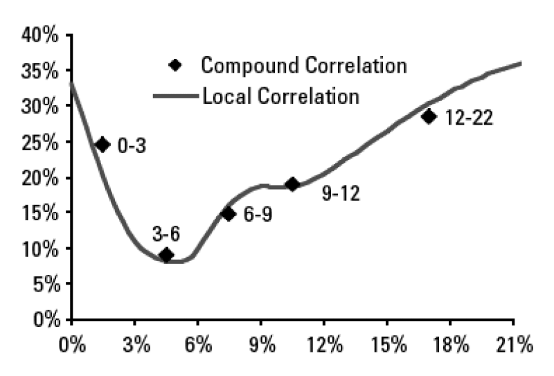
The relationship between local and marginal compound correlation is of no practical use in itself, because tiny CDO tranches are not traded on the market. However, this relationship is extremely useful because it gives a concrete meaning to local correlation, as the correlation of a tiny CDO tranche. Below is an example of the local correlation curve obtained with this method. It shows that the local correlation curve is close to the compound correlation market data.

Limitations Of The Analysis
We made the assumption that base correlation is the level of correlation that fits the value of the floating leg of a given equity piece. This is not entirely true. CDOs traded on the market ('American' CDOs) generally decrease the premium paid to investors after a credit event. Base correlations are defined as correlations that fit to market spreads of traded CDOs, and not to their floating leg. There is a DV01 factor between the floating leg and the spread of a CDO, and this DV01 is a constant only on so-called European CDOs. So, our analysis holds for European CDOs.
Second, the large-pool approximation used for making the transition from distribution of losses into conditional default risk holds only on a large and homogeneous portfolio. This is hardly the case for real-life CDOs. This approximation is useful to get a full and intuitive understanding of the mechanism, and as we will see in a coming article, it can be used as a starting point for a more precise numerical scheme.
This week's Learning Curve was written by Julien Turc,Philippe Very,David Benhamou, andBenjamin Herzog, quantitative credit strategy officials at SG Corporate & Investment Bankingin Paris.


